TL;DR
NeRFs represent a 3D scene as a fully-connected deep network
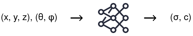
Map any 3D location [math](x, y, z)[/math] and viewing direction [math](\theta, \phi)[/math] to a volume density value [math]\sigma[/math] and a colour (emitted radiance) [math]c=(r, g, b)[/math] at that location that can then be used to render a novel view with classical volume rendering techniques
How it works
Sample
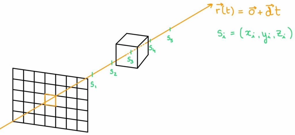
Trace a camera ray [math]r(t)[/math] through the currently shaded pixel into the scene and sample [math]s_0, s_1, …, s_N[/math] along it, [math]s_i=(x_i, y_i, z_i)[/math]
Infer
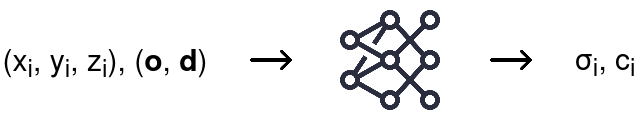
For each sample, have the trained network infer its corresponding density [math]\sigma_i[/math] and colour [math]c_i[/math]
Accumulate
Use classical volume rendering to accumulate colours and densities into the colour of the shaded pixel
[math] C(r) = \int_{t_n}^{t_f} [/math] [math] T(t) [/math] [math] \sigma(r(t)) [/math] [math] c(r(t), d) [/math] [math] dt [/math]
Accumulated transmittance from [math]t_n[/math] to [math]t[/math]
Volume density at [math]r(t)[/math]
Colour at [math]r(t)[/math] when looking in the direction of [math]d[/math]
Backpropagate
TODO
Why it works
- Volume rendering is naturally differentiable (it’s literally the result of an integral) → use gradient descent to train the model by minimising error between observed images of the scene and corresponding rendered views
- Positional encoding
- Issue: basic implementation of the above does not capture high frequency details (lots of sharp changes over a small area of the image) because the input is only 5D
- Solution: project the 5D input into a higher dimensional space through sin and cos functions to represent both coarse and fine details
- Hierarchical volume sampling
- Issue: basic implementation of the above requires a lot of samples per camera rays to accurately capture a scene since they are sampled at random
- Solution: use two networks: a coarse one that takes as input samples taken coarsely at random along the ray, use the densities it outputs to drive a finer sampling that will serve as input to a fine network which will give the final output densities and colours used for rendering
Why it’s cool
- Can model complex geometry and non-Lambertian surfaces (colour of the surface changes depending on the viewing direction)
- Gives an extremely compact representation of a 3D scene: NeRF optimised weights need less memory than the input JPEG images it trained on
- Gives a continuous representation of a 3D scene (prior related work is discrete)
Related Work
Implicit 3D shape representations
Represent continuous 3D shapes implicitly through functions mapping any spatial points to some meaningful value
Using ground truth geometry
How it works
Optimise a network to map any spatial point [math]xyz[/math] to:
- Signed distance functions: how far that point is from the closest surface of the shape
- Minimise MSE loss between predicted and ground truth values at sampled 3D coordinates (regression)
- SDF are continuous and differentiable so we can optimise on them
- Surface can be extracted via marching cubes (SDF = 0 for points on the surface)
- Occupancy fields: maps [math]xyz[/math] to [math]\sigma \in [0, 1][/math] indicating occupancy probability of the point (whether it’s inside the shape (1) or outside (0))
- Minimise a binary cross-entropy loss between predicted occupancy and ground truth label (binary classification, easier than regressing SDF: easier to define labels, more stable gradients, faster convergence)
- Surface can be extracted via marching cubes (occupancy probability is 0.5 for points on the surface)
Marching cubes algorithm
Convert an implicit surface into a polygonal mesh
- Sample the 3D space at regular intervals
- Evaluate the function representing the implicit surface (SDF, occupancy field, …) at each grid point
- Identify grid cells where the function value crosses the threshold value (0 for SDF, 0.5 for occupancy field) across corners (means the surface passes through that cell)
- Approximate the surface within these cells according to a precomputed lookup table
- For each cube in the grid, you have 8^2=256 possible configurations (SDF/occupancy for each of the 8 corners is over or below the threshold) and for each configuration you use a precomputed lookup table to know how to draw triangles within that cell to approximate the surface
Limitations
- Requires ground truth geometry to optimise on
Leveraging differentiable rendering functions
How it works
Formulate differentiable rendering functions to use the above methods with ground truth images rather than ground truth geometry
Numerical method and implicit differentiation example
- Cast a camera ray [math]r(t) = o + td[/math] through the image plane into the 3D scene and numerically search for the point [math]t*[/math] where the ray intersects the implicitly defined surface (ex: for application to the occupancy fields [math]f(r(t*))=0.5[/math])
- Once you find [math]t*[/math], you ask the network to predict the colour at that point, compare to the ground truth colour of the image, and then you want to backpropagate through this loss [math]L[/math] to update the neural network
- The iterative numerical method used to find t* is not differentiable, so use implicit differentiation on the constraint [math]f(r(t*))=0.5[/math] to compute [math]\frac{dL}{d \theta}[/math]
Limitations
- Limited to simple shapes with low geometric complexity → over smoothed renderings
View synthesis and image-based rendering
Synthesise high-quality photorealistic novel views of a scene from a set of input RGB images of that scene
Light field sample interpolation
How it works
- The light field represents all the light rays in a scene: colour and intensity as a function of pixel position and viewing direction
[math]L(u, v, s, t)[/math]
- [math](u, v)[/math]: image coordinates
- [math](s, t)[/math]: viewing directions
- To generate light field values for unseen [math](s, t)[/math] pairs, we interpolate colour and intensity values for the unseen pair from nearby sampled views to generate a novel view
Limitations
- Requires dense and regularly spaced input views
- Assumes scene continuity: locally smooth, surfaces and colours change gradually across views → miss high frequency details and sharp edges
Scene Representation Networks
How it works
Represent scenes as continuous functions that map world coordinates to a feature representation of local scene properties
For each pixel in the novel view to be rendered:
- Trained depth MLP predicts depth at which the ray hits a surface: takes as input ray origin and direction, camera parameters and scene code (latent vector representing the current scene) and outputs a predicted t (ray paramter) where closest intersection occurs
- Can train an input images to scene code encoder -> SRN is generalisable across different scenes
- Trained scene MLP predicts RGB colour (and additional properties like occupancy, visibility, …) from intersection point in space and scene code
Limitations
- Learned ray marching is less stable than volume rendering used by NeRF
- View independent: does not consider viewing direction when predicting colour -> can’t predict specularities or reflections
Sampled volume representations
Learn volumetric scene parameters at sampled points in the scene
Colouring voxel grids
Use observed images to directly colour voxel grids
- Define a regular grid of 3D voxels inside a 3D bounding volume that encloses the scene
- For each voxel, use the known camera intrinsics and extrinsics to project it into each image, define the colour of this voxel as the average of the colours of all corresponding pixels over the input images
Limitations: assumes colour does not depend on viewing direction, need camera parameters
Sampled volume representations
Train scene-independent deep network that predicts a sampled representation from a set of input images and use alpha compositing or learned compositing to render novel views
Alpha compositing (classic volume rendering)
Render volumetric representations (we have colour and density at any given point in space)
Combine predicted colour and density samples through a fixed equation
To render an image using predicted colour [math]c_i[/math] and density [math]\sigma_i[/math] values at a given point and viewing direction, we do the following for each camera ray:
- Sample points along the ray in the 3D space
- Predict colour and density at these points
- Blend them using the standard volume rendering equation:
- [math]C = \sum_{i}T_i alpha_i c_i[/math]
- Opacity [math]\alpha_i = 1 – \text{exp}(-\sigma_i \delta_i)[/math]
- Transmittance [math]\T_i=\text{exp}(- \sum_{j=1}^{i-1} \sigma_j \delta_i)[/math]
- Distance between adjacent samples [math]\delta_i[/math]
- [math]C = \sum_{i}T_i alpha_i c_i[/math]
Learned compositing (neural volume rendering)
Render volumetric or sampled representations (we have value at any given point in space and viewing direction)
Train a network to combine them
- More expressive than alpha compositing:
- Can model non-Lambertian effects (reflections, specular highlights)
- Can learn to handle occlusions, depth ambiguity
- Look more into it
Relevant example is “Neural Volumes: Learning Dynamic Renderable Volumes from Images” (SIGGRAPH 2019)
Limitations
- Can’t scale to higher resolution imagery because of poor time and space complexity due to discrete sampling
- NeRF encodes a continuous volume -> requires way less storage than sampled volumetric representations
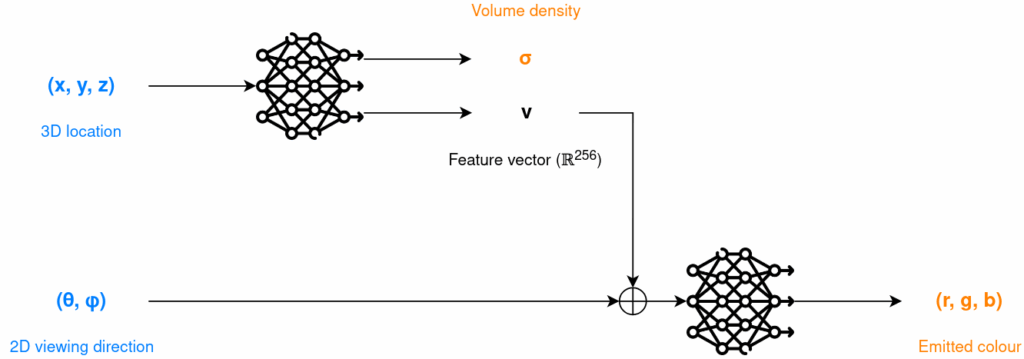
Architecture
Predict volume density from coordinates only and emitted colour from full input to ensure multiview consistency
What does this represent? Do both coarse and fine nets have this architecture?
Volume Rendering with Radiance Fields
Use classical volume rendering principles to render the colour of any ray passing through the scene using predicted local density and colour
To render a novel view, we need to shade every pixel of the image: trace a ray through each pixel and estimate the colour of this ray.
Volume rendering equation
Volume rendering equation gives the expected colour [math]C(r)[/math] of a camera ray [math]r(t)=o+td[/math] with near and far bounds [math]t_n[/math] and [math]t_f[/math]
[math] C(r) = \int_{t_n}^{t_f} [/math] [math] T(t) [/math] [math] \sigma(r(t)) [/math] [math] c(r(t), d) [/math] [math] dt [/math]
| [math] T(t) = \text{exp} ( – \int_{t_n}^{t} \sigma(r(s)) ds ) [/math] | [math] \sigma(r(t)) [/math] | [math] c(r(t), d) [/math] |
| Accumulated transmittance from [math]t_n[/math] to [math]t[/math] | Volume density at [math]r(t)[/math] | Colour at [math]r(t)[/math] when looking in the direction of [math]d[/math] |
| “How much stuff have we encounted along the ray up until the current point?” → is a function of previous densities | “How much stuff is there at the current point?” | “What colour is the stuff at the current point?” |
- The inside of the integral answers the question “How much of this [math] c(r(t), d) [/math] colour should I see at point [math]r(t)[/math], considering how much stuff is in front of that point and how much stuff of that colour actually is at that point?”
- The whole integral answers the question: “How much of each colour along the ray should I see?”
Quadrature estimate
Estimate the result of the volume rendering equation as a sum of samples
[math] \hat{C}(r) = \sum_{i=1}^{N} [/math] [math]T_i[/math] [math] (1 – \text{exp}(- \sigma_i \delta_i)) [/math] [math]c_i [/math]
| [math] T_i = \text{exp}(- \sum_{j=1}^{i-1} \sigma_j \delta_i) [/math] | [math] (1 – \text{exp}(- \sigma_i \delta_i)) [/math] | [math] c_i [/math] |
| Accumulated transmittance for samples 1 to [math]i[/math] | Volume density at [math]r(t)[/math] | Colour at [math]r(t_i)[/math] when looking in the direction of [math]d[/math] |
[math]\delta_i = t_{i+1} – t_i[/math] is the distance between two adjacent samples
[math] \hat{C}(r)[/math] is trivially differentiable and reduces to traditional alpha compositing with alpha values [math] \alpha_i = 1 – \text{exp}(- \sigma_i \delta_i) [/math]
Optimising a Neural Radiance Field
Positional encoding
Allow the input to represent both fine and coarse grained details
Initial input coordinates (position + viewing direction) does not allow for representation of high-frequency variation in colour and geometry (deep networks are biased towards learning lower frequency functions) -> map inputs to higher dim space before passing them to network to have better fitting of data that contains high frequency variation (rapid changes over space, data fluctuates a lot and quickly, ex: images with lots of sharp edges or fine details)
Reformulate network function [math]F_{\Theta}[/math] as composition:
[math]F_{\Theta} = F’_{\Theta} \circ \gamma[/math]
- [math]F’_{\Theta}[/math]: regular MLP, learned
- [math]\gamma: \mathbb{R} \rightarrow \mathbb{R}^{2L} [/math], not learned
[math]\gamma(p) = (\sin(2^0\pi p), \cos(2^0\pi p), …, \sin(2^{L-1}\pi p), \cos(2^{L-1}\pi p))[/math]
[math]\gamma(\cdot)[/math] applied separately to three coordinates values x, y, z normalised to lie in [-1, 1] and three components of cartesian unit vector [math]\vec{d}[/math] corresponding to viewing direction (lies in [-1, 1] by construction).
Visual understanding
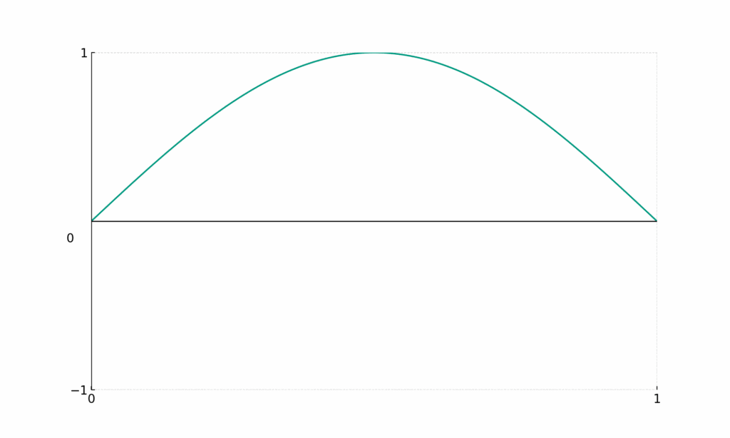
[math]\sin{(\pi x)}[/math]
- Encodes coarse details
- Big change in [math]x[/math] induces small change in [math]y[/math]
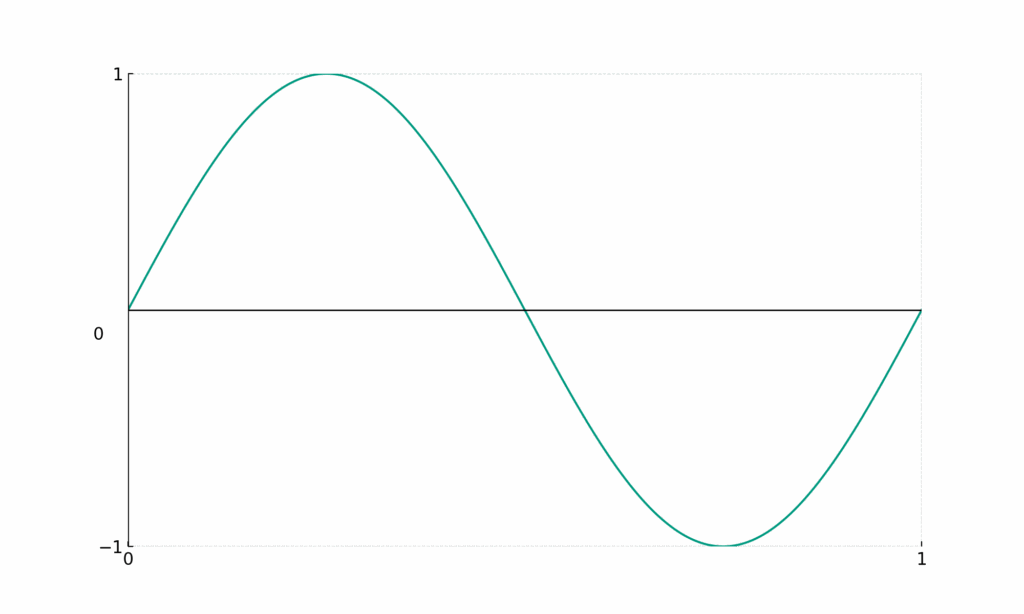
[math]\sin{(2 \pi x)}[/math]
- Encodes slightly finer details
- Big change in [math]x[/math] induces a bit more change in [math]y[/math]
…
…
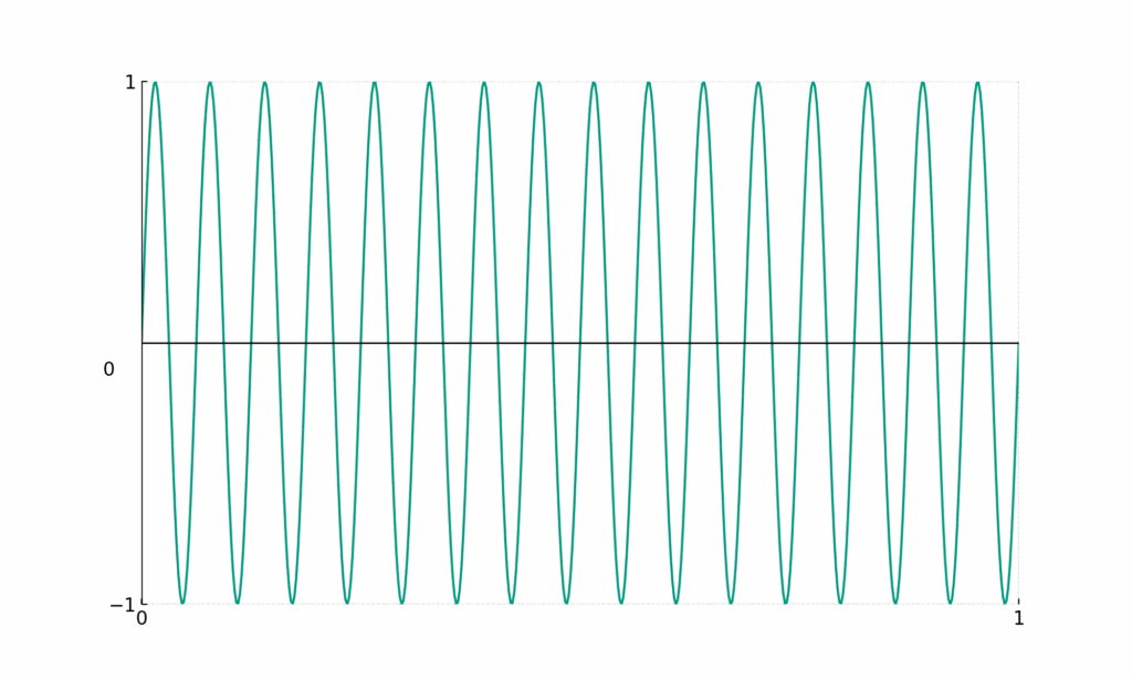
[math]\sin{(32 \pi x)}[/math]
- Encodes fine details
- Even a small change in [math]x[/math] induces a big change in [math]y[/math]
Hierarchical volume sampling
Inefficient to evaluate network at [math]N[/math] query points along each camera ray: free space and occluded regions sampled repeatedly while they don’t contribute to rendered image -> use a hierarchical representation: allocate samples proportionally to expected effect on final rendering (== “sample with a preference for areas where there’s actual stuff to see”)
Optimise two networks instead of one: “coarse” and “fine” one
First sample [math]N_c[/math] locations through stratified sampling and evaluate coarse network at these locations according to previously mentioned equation:
[math] \hat{C}(r) = \sum_{i=1}^{N} T_i (1 – \text{exp}(- \sigma_i \delta_i))c_i [/math]
With
[math]T_i=\text{exp}(- \sum_{j=1}^{i-1} \sigma_j \delta_i)[/math]
Gives us colour from the coarse network: [math]\hat{C}_c(r)[/math]
Use the coarse samples to evaluate where we should sample with a finer grain.
Rewrite it as weighted sum of sampled colours [math]c_i[/math] along the ray (simple rewriting of the above really):
[math]\hat{C}_c(r) = \sum_{i=1}^{N_c} w_i c_i [/math]
[math]w_i = T_i(1-\text{exp}(-\sigma_i \delta_i)[/math]
Normalise the weights:
[math]\hat{w}_i = \frac{w_i}{\sum_{j=1}^{N_c} w_j}[/math]
And we get a piecewise-constant PDF along the ray.
Sample second set of [math]N_f[/math] locations from this distribution using inverse transform sampling, evaluate fine network at union of first and second set of samples and compute final rendered colour of the ray [math]\hat{C}_f(r)[/math] using always the same equation
[math] \hat{C}(r) = \sum_{i=1}^{N} T_i (1 – \text{exp}(- \sigma_i \delta_i))c_i [/math]
But using all [math]N_c + N_f[/math] samples -> allocate more samples to region that have visible content
Optimise both coarse and fine networks jointly
The output view is the output of the fine network
Fine sampling is basically educated sampling
Stratified sampling
- Partition [math][t_n, t_f][/math] into [math]N[/math] evenly-spaced bins, draw one sample uniformly at random from each bin
[math]t_i \sim U [ t_n + \frac{i-1}{N}(t_f – t_n), t_n + \frac{i}{N}(t_f – t_n) ][/math]
- Enables a continuous scene representation: MLP is being evaluated at continuous positions over the course of optimisation
Objective
[math]L = \sum_{r \in R} [ || [/math] [math] \hat{C}_c(\vec{r}) [/math] [math] – [/math] [math]C(\vec{r}) [/math][math] ||_2^2 + || [/math][math] \hat{C}_f(\vec{r}) [/math] [math] – C(\vec{r}) ||_2^2 ] [/math]
| [math]R[/math] | [math]\hat{C}_c(\vec{r})[/math] | [math]C(\vec{r})[/math] | [math]\hat{C}_f(\vec{r})[/math] |
| Set of all ray shooted through the ground truth image pixels | Coarse network prediction | Ground truth colour | Fine network prediction |
Sources
- Mildenhall, B., Srinivasan, P. P., Tancik, M., Barron, J. T., Ramamoorthi, R., & Ng, R. (2020). NeRF: Representing Scenes as Neural Radiance Fields for View Synthesis. arXiv:2003.08934
- NeRF: Representing Scenes as Neural Radiance Fields for View Synthesis (ML Research Paper Explained)
- A Brief Introduction to Neural Radiance Fields | CESCG Academy 2023