Introduction

Graphics and discretisation

Raster graphics/displays: images and screens that use a two-dimensional array of pixels to represent or display images
Colour quantisation: find the closest possible matching colour from the palette to the colour you ideally want and display this matching colour -> banding if not enough colours available, (continuous gradients of colour tones, see below)

Aliasing: occurs when having to break down a continuous function into discrete values. Small details, smaller than a pixel, can’t be displayed properly
Vector graphics vs bitmap graphics: do not store pixels but represent the shape of objects and their colours using mathematical expressions -> shapes can be rendered on the fly at the desired resolution

Geometry representation

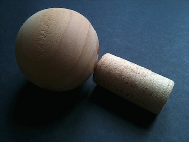
Implicit surfaces: objects for which the surface can be described with an equation, ex: x² + y² + z² = r²
Parametric surfaces: each coordinate is given by a parameterised formula, ex: (x, y, z)=(r*cosθ*sinϕ, r*sinθ*sinϕ, r*cosϕ)
Rendering primitive: convert the surface to a representation made of only the same geometry primitive to achieve better performance
- Triangle is preferred: coplanar, indivisible, the barycentric coordinates maths is simple and robust.
- Extensive research to find best algorithm for computing ray-triangle intersections
- Modern hardware is optimised for triangles

The rendering process: two essential steps

Visibility problem

Define which geometry is visible at the pixel we’re considering

Foreshortening effect: objects further away from our eyes appear smaller than those closer
Hidden surface elimination/determination, occlusion culling: determining which surfaces and parts of surfaces are not visible from the viewpoint, can be solved by rasterisation (z-buffer and painter’s algorithms) or ray-tracing

Shading

The simulation of light (light transport) and the simulation of the appearance of objects (shading)

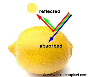
Light emitted by sources travels straight until meets an object, then some is reflected and some is absorbed

Absorption: gives objects their colour, a black object absorbs all light colors, while a white object reflects them all
Reflection: outgoing direction is a reflection of the incoming direction with respect to the normal

Reflection happens at the object level but scattering (re-emission of incoming photon to a random direction) happens at the atomic level -> shaders model the light interaction with materials at the microscopic level.

The Visibility Problem

Perspective projection

Projecting 3D shapes onto the surface of a canvas and determining which parts of these surfaces are visible from a given point of view.

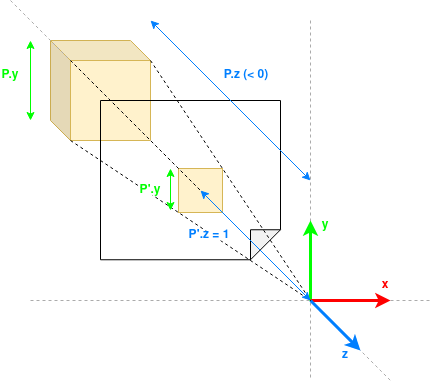
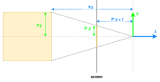
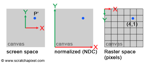
Projected points coordinates are in screen space. Normalising them to the 0,1 range, we get the coordinates in NDC (Normalised Device Coordinates) space. We can multiply them by the dimensions of the image to get the coordinates raster space (in the image as a 2D grid of pixels with origin in the top-left corner of the image).

Coordinate spaces

Object space

Local coordinate system of a 3D object
Origin at center/corner of the object, range between 0 and 1 or -1 and 1
Useful to model, transform object independently (scale, rotate, …)

World space

Shared coordinate system for entire 3D scene
Useful to place objects relative to each other

View/Camera space

Coordinate system from the camera’s viewpoint: camera at the origin looking down he negative z-axis
Useful to convert the scene so that everything is relative to the camera

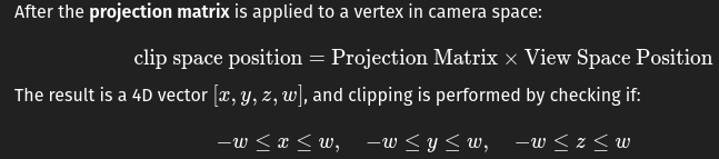
Clip space

Coordinate space after a vertex has been transformed by the projection matrix (perspective or orthographic), but before the perspective divide
Space where the GPU determines whether a vertex is inside or outside the view frustum (whether to “clip” it or not)

Normalised Device Coordinates (NDC)

Coordinates normalized into a cube where all axes range from -1 to 1
Useful to determine whether geometry is in the view frustum
Basically clip coordinates / w

Screen space

2D coordinates on your screen, in pixels
Range from 0 to screen width/height

Raster space

Discrete grid of pixels on the screen
Useful to run pixel shaders and per-pixel operations (texturing)

From	To	Transformation	Description
Object Space	World Space	Model Matrix (M)	Places the object into the world (translation, rotation, scaling).
World Space	View Space	View Matrix (V)	Transforms everything relative to the camera’s position and orientation.
View Space	Clip Space	Projection Matrix (P)	Applies perspective or orthographic projection.
Clip Space	NDC	Perspective Divide (divide by w)	Normalizes coordinates into the range [-1, 1] for x, y, z.
NDC	Screen Space	Viewport Transform	Maps from NDC to pixel coordinates on the screen.
Screen Space	Raster Space	Rasterization (Discrete Pixel Sampling)	Converts continuous screen coordinates to actual pixel fragments.

Projection matrix

Perspective projection matrix: when applied to points on the geometry, projects them onto the screen

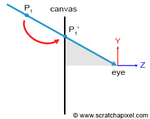
Rasterisation: project P onto the screen to compute P’ -> need the projection matrix
Ray-tracing: trace a ray passing through P’ and search for P -> projection matrix not needed

Rasterisation solution

Rasterisation is moving a point along a line that connects a point on a geometry surface, to the eye until it lies on the canvas surface

Several points can project onto the same point on the canvas but the only visible one is the closest to the eye -> visibility problem

Depth sorting algorithm

Project all points onto the screen
- For each projected point, convert coordinates from screen space to raster space
- Determine the pixel to which the point maps and store the distance from that point to the eye in the depth list of that pixel
Sort the points in each pixel’s list in order of increasing distance -> point visible for a given pixel is the first point in its depth list

Well-known depth sorting algorithms: z-buffering algorithm, painter algorithm, newell’s algorithm

Ray-tracing solution

Ray-tracing starts with the pixel and converts it into a point on the image plane.

Trace a ray from the eye passing through the center of the pixel and extending it into the scene
If that ray intersects with an object then this intersection point is the point visible through that pixel -> solve the visibility problem by directly tracing rays from the eye into the scene

Rasterisation vs ray-tracing solutions

Ray-tracing is more complicated because we have to solve ray-geometry intersection problems.
Ray-tracing is slower and the render time increases linearly with the amount of geometry in the scene: have to check whether any given ray intersects any of the triangles in the scene
Acceleration structures can alleviate cost of ray-tracing: divide the space into subspaces
- Test if a ray intersects with a given subspace before testing if it intersects with objects in this subspace
- Issues with acceleration structures:
  - Building takes time -> impractical in real-time scenarios where a new structure needs to be built for each frame
  - Takes space in memory -> less space for geometry -> can render less geometry with ray-tracing than with rasterisation
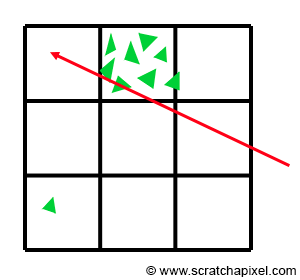
  - Finding an good acceleration structure that subdivides the space in a practical way is difficult, example below of a situation where it’s difficult to find a good subdivision of space:

Light Simulation

Real-world light effects

Reflection

Light interacts with perfect mirror-like surfaces -> reflected back in the environment in a predictable direction given by the law of reflection: angle of reflection of a ray departing a surface equals the angle of incidence at which the incoming ray strikes the surface. around the normal to the surface.

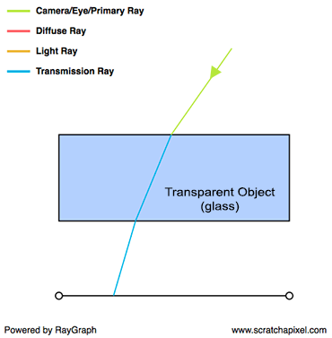
Transparency

Transparent object reflect and refract light.

Snell’s law gives the direction of refraction
Fresnel equations specify the proportions of light that are reflected and refracted

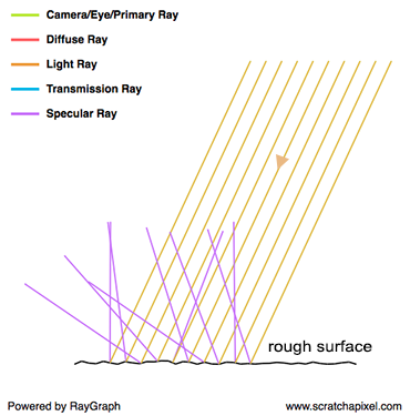
Glossy or specular reflection (scattering)

Glossy/specular reflection == is not perfectly reflective and not perfectly diffuse, glossiness == roughness

Also referred as scattering

Diffuse reflection

Diffuse surface is the opposite of a perfeclty reflective surface. Incident light is equally spread in every direction above the point of incidence and as a result, a diffuse surface appears equally bright from all viewing directions -> the direction of incidence does not affect the light rays’ outing directions

Subsurface scattering

Subsurface scattering == translucency: light travels through the material, changing direction along its path, exiting object at a different location and direction

Indirect lighting (indirect diffuse)

Some part of the surface is not facing any light source, but other illuminated surfaces (here, the floor) reflects light back in on them -> indirect lighting

Caustics (indirect specular)

Reflective objects can indirectly illuminate other objects: concentrate light rays into specific lines or patterns

Soft shadows

Soft shadows are unrelated to material, purely geometric problem to simulate

Light transport and shading

Light effects can be categorised into two groups:

Relate to the appearance of objects: reflection, transparency, specular reflection diffuse reflection, subsurface scattering -> shading
Relate to the amount of light an object receives: indirect diffuse, indirect specular, soft shadows -> light transport

Shading

Interaction between light and matter, everything that happens to light from the moment it reaches an object to the moment it departs

Light transport

Studies journey of light as it bounces from surface to surface, focuses on the paths light rays follow as they move from light source to observer

Global illumination

Global illumination = ability to simulate both direct and indirect lighting effects

Expensive: simulating indirect lighting in addition to direct lighting requires not twice as many rays (compared to the number used for direct lighting) but orders of magnitude more: this effect is recursive, making indirect lighting a potentially very expensive effect to simulate.

“Naive” backward ray tracing is clearly not the solution to everything, and you might look for alternative methods. Photon maps are a good example of a technique designed to efficiently simulate caustics

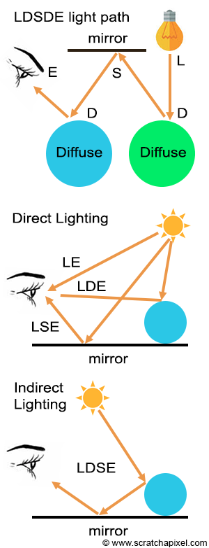
Light Transport

Light paths are defined by all the successive materials with which the light rays interact on their way to the eye.

LE is the smallest possible path
LDE or LSE are direct illumination paths
L(D|S)*E are indirect illumination paths

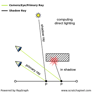
Ray tracing main idea: trace a ray from the eye (primary ray) and check if it intersects geometry. If it does we need to compute how much light arrives at this intersection P directly from the light sources (direct contribution) and how much light arrives indirectly as a result of reflection on other surfaces (indirect contribution).

Direct contribution

Trace a ray from intersection point to light source (shadow ray)
If it intersects another object, then initial point is in the shadow of this object

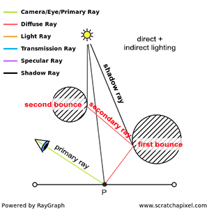
Indirect contribution

Need to spawn secondary rays from the intersection point into the scene

If secondary ray intersects other surface, need to determine how much light is reflected towards the intersection point along these rays -> recursive process: cast again a shadow ray and a secondary ray from this intersection:

Compute the amount of light arriving at the point of intersection between the secondary ray and the surface
Measure how much of that light is reflected by the surface towards the intersection point (depends on surface properties, done with shaders)

Number of such bounces may be infinite -> Monte Carlo ray tracing: shooting a few rays to approximate the exact amount of light arriving at a point

Whitted-style ray tracing (Unidirectional path tracing)

Simple light transport model that only accounts for direct illumination, perfect reflection, refraction and sharp shadows. At intersection point, you only compute local illumination, cast a shadow ray, and cast a reflection or refraction ray if the surface requires it -> light only bounces once -> no global illumination

Light transport algorithms

Try to solve what can’t be solved by unidirectional path tracing, mostly the LS+DE problem (bounces from light to multiple specular surfaces before a diffuse one and the eye. Can be categorised into two groups

Not using ray tracing: photon/shadow mapping, radiosity, …
Exclusively using ray tracing

-> Ray tracing is not the only way to solve global illumination

Shading

Model light real world light interactions that are too complex to simulate with light transport approach

Albedo vs Luminance vs Chromaticity

Albedo: what colour the object is
- True colour without any lighting involved
- Can be measured precisely for an object
Luminance: how bright the object looks
- Depends on how much light energy the surface reflects into your eye: bright in direct sunlight but dark or even black at night, but albedo has not changed
Chromaticity: what hue/saturation the object has
- Colour “type” without brightness, “what kind of colour is it? red, green, blue? how pure?”
- Albedo includes brightness while chromaticity is normalised to show hue/saturation only

What is shading

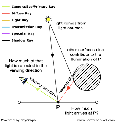
Brightness of a point P on the surface of an object under lighting conditions needs to account for:

How much light falls on the object at this point: contributions from light sources (direct lighting) and other surfaces (indirect lighting) -> light transport issue
How much light is reflected from this point in the viewing direction -> shading issue, more complex, depends on:
- Viewing direction: diffuse surfaces appear equally bright from all viewing angles but specular surfaces do not, most objects are a mix of the two
- Incoming light’s direction:

Shader

Takes incident light direction and viewing direction as input and returns the fraction of light reflected by the surface for these directions

[math]\text{ratio of reflected light}=\text{shader}(\omega_i, \omega_O)[/math]